13. Perceptrons II
Perceptron
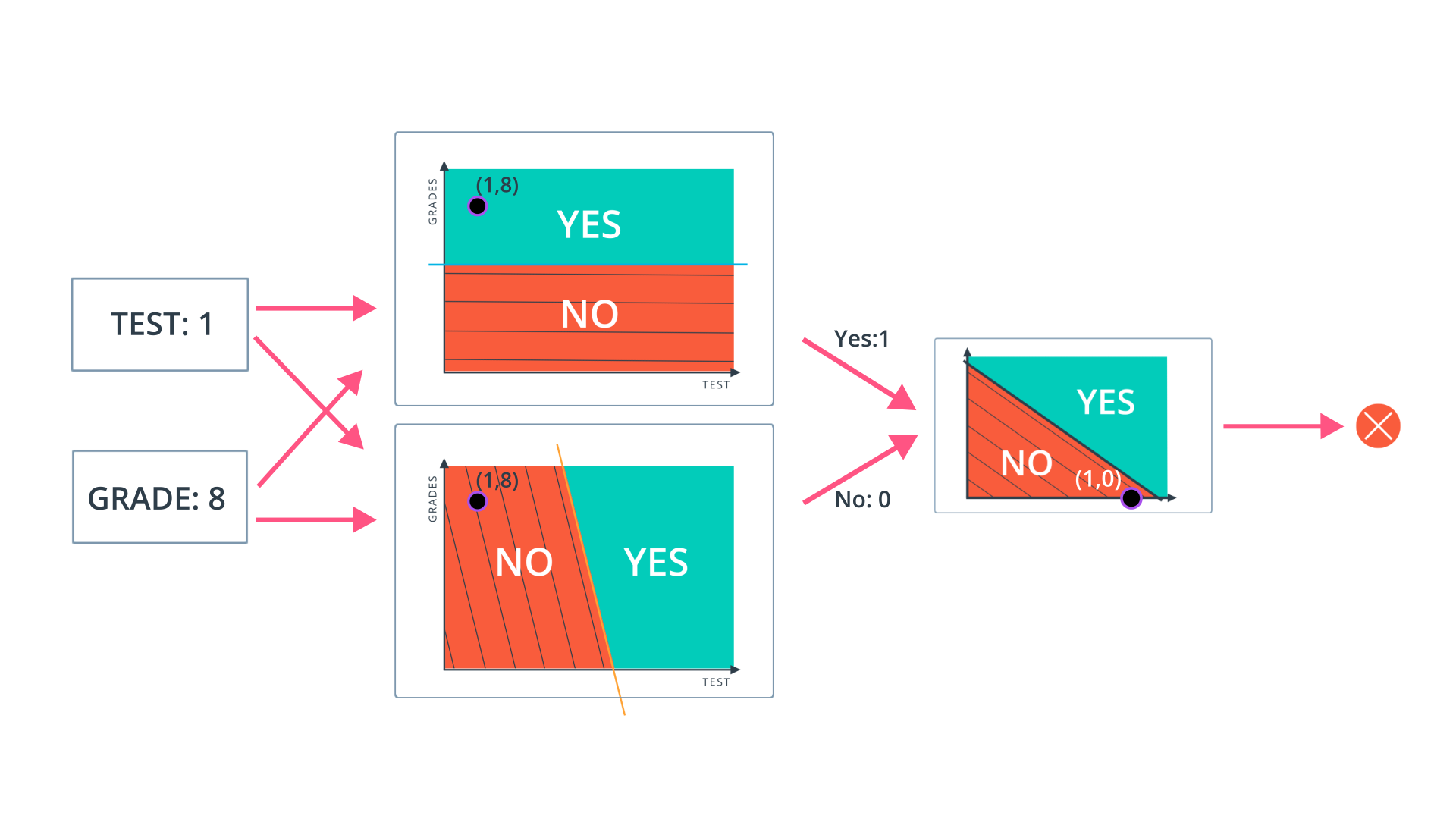
Now you've seen how a simple neural network makes decisions: by taking in input data, processing that information, and finally, producing an output in the form of a decision! Let's take a deeper dive into the university admission example to learn more about processing the input data.
Data, like test scores and grades, are fed into a network of interconnected nodes. These individual nodes are called perceptrons , or artificial neurons, and they are the basic unit of a neural network. Each one looks at input data and decides how to categorize that data. In the example above, the input either passes a threshold for grades and test scores or doesn't, and so the two categories are: yes (passed the threshold) and no (didn't pass the threshold). These categories then combine to form a decision -- for example, if both nodes produce a "yes" output, then this student gains admission into the university.
Let's zoom in even further and look at how a single perceptron processes input data.
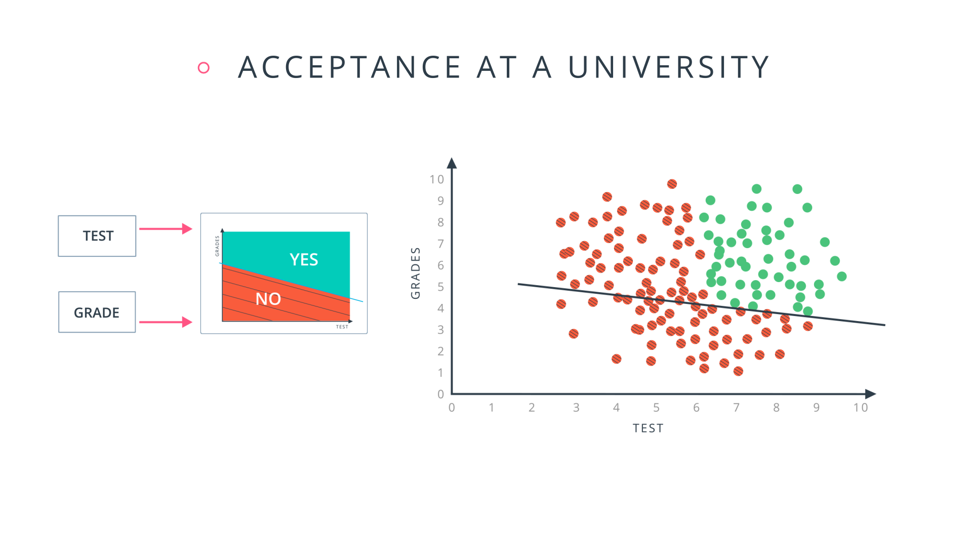
The perceptron above is one of the two perceptrons from the video that help determine whether or not a student is accepted to a university. It decides whether a student's grades are high enough to be accepted to the university. You might be wondering: "How does it know whether grades or test scores are more important in making this acceptance decision?" Well, when we initialize a neural network, we don't know what information will be most important in making a decision. It's up to the neural network to learn for itself which data is most important and adjust how it considers that data.
It does this with something called weights .
Weights
When input comes into a perceptron, it gets multiplied by a weight value that is assigned to this particular input. For example, the perceptron above has two inputs,
tests
for test scores and
grades
, so it has two associated weights that can be adjusted individually. These weights start out as random values, and as the neural network network learns more about what kind of input data leads to a student being accepted into a university, the network adjusts the weights based on any errors in categorization that results from the previous weights. This is called
training
the neural network.
A higher weight means the neural network considers that input more important than other inputs, and lower weight means that the data is considered less important. An extreme example would be if test scores had no affect at all on university acceptance; then the weight of the test score input would be zero and it would have no affect on the output of the perceptron.
Summing the Input Data
Each input to a perceptron has an associated weight that represents its importance. These weights are determined during the learning process of a neural network, called training. In the next step, the weighted input data are summed to produce a single value, that will help determine the final output - whether a student is accepted to a university or not. Let's see a concrete example of this.
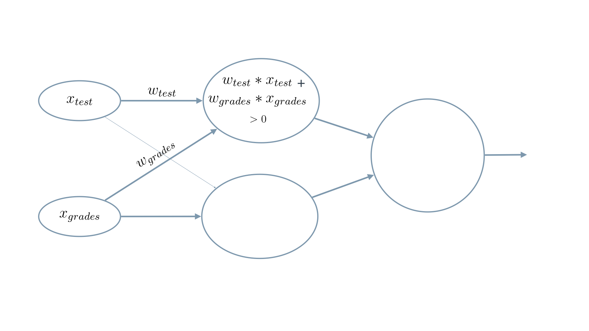
We weight
x_test
by
w_test
and add it to
x_grades
weighted by
w_grades
.
When writing equations related to neural networks, the weights will always be represented by some type of the letter w . It will usually look like a W when it represents a matrix of weights or a w when it represents an individual weight, and it may include some additional information in the form of a subscript to specify which weights (you'll see more on that next). But remember, when you see the letter w , think weights .
In this example, we'll use
w_{grades_{}}
for the weight of
grades
and
w_{test}
for the weight of
test
.
For the image above, let's say that the weights are:
w_{grades} = -1, w_{test} = -0.2
. You don't have to be concerned with the actual values, but their relative values are important.
w_{grades_{}}
is 5 times larger than
w_{test}
, which means the neural network considers
grades
input 5 times more important than
test
in determining whether a student will be accepted into a university.
The perceptron applies these weights to the inputs and sums them in a process known as linear combination . In our case, this looks like w_{grades} \cdot x_{grades} + w_{test} \cdot x_{test} = -1 \cdot x_{grades} - 0.2 \cdot x_{test} .
Now, to make our equation less wordy, let's replace the explicit names with numbers. Let's use 1 for grades and 2 for tests . So now our equation becomes
w_{1} \cdot x_{1} + w_{2} \cdot x_{2}
In this example, we just have 2 simple inputs: grades and tests. Let's imagine we instead had
m
different inputs and we labeled them
x_1, x_2, …, x_m
. Let's also say that the weight corresponding to
x_1
is
w_1
and so on. In that case, we would express the linear combination succintly as:
\sum_{i=1} ^ m w_i \cdot x_i
Here, the Greek letter Sigma \sum is used to represent summation . It simply means to evaluate the equation to the right multiple times and add up the results. In this case, the equation it will sum is w_i \cdot x_i
But where do we get w_i and x_i ?
\sum_{i=1} ^ m means to iterate over all i values, from 1 to m .
So to put it all together, \sum_{i=1} ^ m w_i \cdot x_i means the following:
- Start at i = 1
- Evaluate w_1 \cdot x_1 and remember the results
- Move to i = 2
- Evaluate w_2 \cdot x_2 and add these results to w_1 \cdot x_1
- Continue repeating that process until i = m , where m is the number of inputs.
One last thing: you'll see equations written many different ways, both here and when reading on your own. For example, you will often just see \sum_{i_{}} instead of \sum_{i=1} ^ m . The first is simply a shorter way of writing the second. That is, if you see a summation without a starting number or a defined end value, it just means perform the sum for all of the them. And sometimes , if the value to iterate over can be inferred, you'll see it as just \sum . Just remember they're all the same thing: \sum_{i=1} ^ m w_i \cdot x_i = \sum_{i} w_i \cdot x_i = \sum w_i \cdot x_i .
Calculating the Output with an Activation Function
Finally, the result of the perceptron's summation is turned into an output signal! This is done by feeding the linear combination into an activation function .
Activation functions are functions that decide, given the inputs into the node, what should be the node's output? Because it's the activation function that decides the actual output, we often refer to the outputs of a layer as its "activations".
One of the simplest activation functions is the Heaviside step function . This function returns a 0 if the linear combination is less than 0. It returns a 1 if the linear combination is positive or equal to zero. The Heaviside step function is shown below, where h is the calculated linear combination:
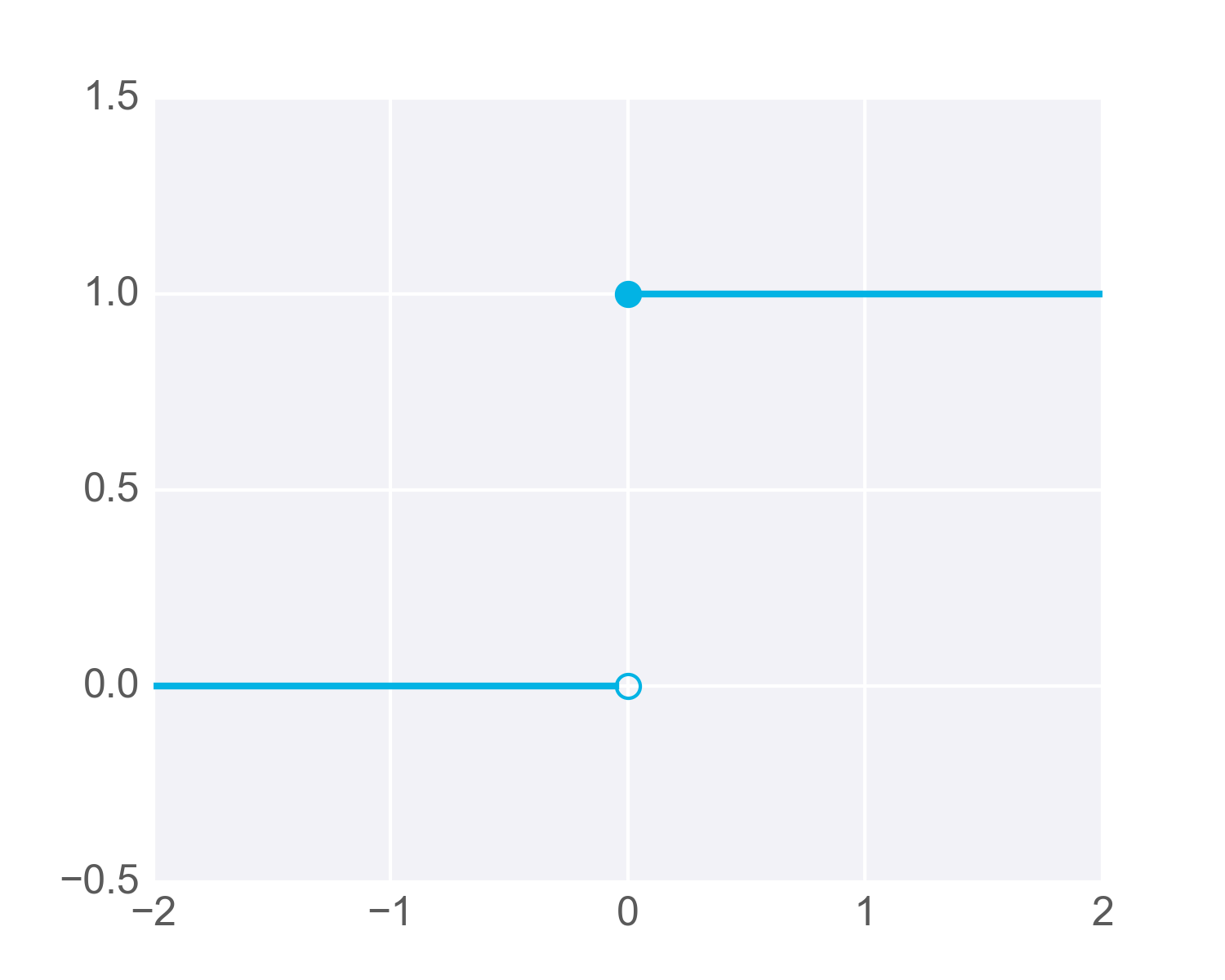
The Heaviside Step Function
In the university acceptance example above, we used the weights w_{grades} = -1, w_{test} = -0.2 . Since w_{grades_{}} and w_{test} are negative values, the activation function will only return a 1 if grades and test are 0 ! This is because the range of values from the linear combination using these weights and inputs are (-\infty, 0] (i.e. negative infinity to 0, including 0 itself).
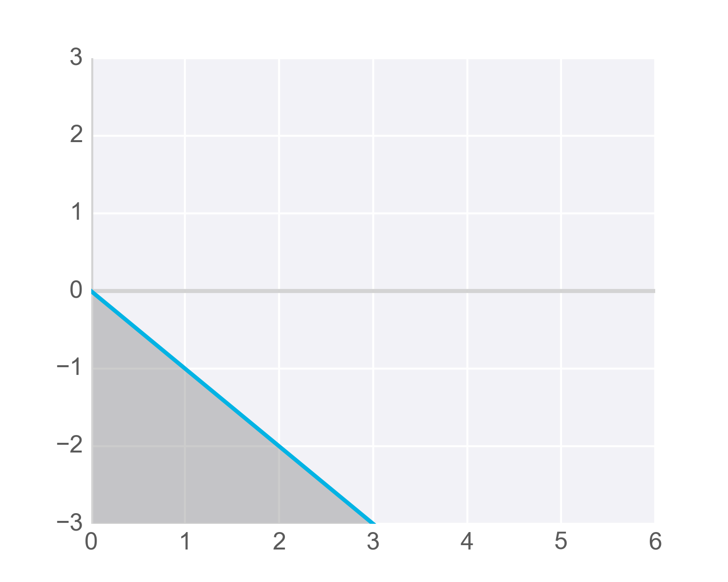
It's easiest to see this with an example in two dimensions. In the following graph, imagine any points along the line or in the shaded area represent all the possible inputs to our node. Also imagine that the value along the y-axis is the result of performing the linear combination on these inputs and the appropriate weights. It's this result that gets passed to the activation function.
Now remember that the step activation function returns 1 for any inputs greater than or equal to zero. As you can see in the image, only one point has a y-value greater than or equal to zero – the point right at the origin, (0, 0) :
Now, we certainly want more than one possible grade/test combination to result in acceptance, so we need to adjust the results passed to our activation function so it activates – that is, returns 1 – for more inputs. Specifically, we need to find a way so all the scores we’d like to consider acceptable for admissions produce values greater than or equal to zero when linearly combined with the weights into our node.
One way to get our function to return 1 for more inputs is to add a value to the results of our linear combination, called a bias .
A bias, represented in equations as b , lets us move values in one direction or another.
For example, the following diagram shows the previous hypothetical function with an added bias of +3 . The blue shaded area shows all the values that now activate the function. But notice that these are produced with the same inputs as the values shown shaded in grey – just adjusted higher by adding the bias term:
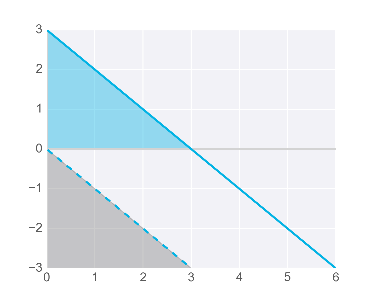
Of course, with neural networks we won't know in advance what values to pick for biases. That’s ok, because just like the weights, the bias can also be updated and changed by the neural network during training. So after adding a bias, we now have a complete perceptron formula:
Perceptron Formula
This formula returns 1 if the input ( x_1, x_2, …, x_m ) belongs to the accepted-to-university category or returns 0 if it doesn't. The input is made up of one or more real numbers , each one represented by x_i , where m is the number of inputs.
Then the neural network starts to learn! Initially, the weights ( w_i ) and bias ( b ) are assigned a random value, and then they are updated using a learning algorithm like gradient descent. The weights and biases change so that the next training example is more accurately categorized, and patterns in data are "learned" by the neural network.
Now that you have a good understanding of perceptrons, let's put that knowledge to use. In the next section, you'll create the AND perceptron from the Neural Networks video by setting the values for weights and bias.